State Space Representation Of A Mass Spring Damper System

Hello,
I plan to write a bunch of posts about simulating dynamic systems using Python.
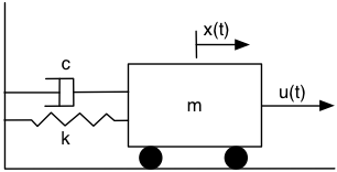
I will be using the mass-spring-damper (MSD) system as an example through those posts so here is a brief description of the typical MSD system in state space.

Mass-Spring-Damper System

Schematic of mass-spring-damper

The differential equation that describes a MSD is:

$latex m \ddot{x} + c \dot{x} + k x = u$

x : position of mass [m] at time t [s]
m : mass [kg]
c  : viscous damping coefficient [N s / m]
k  : spring constant [N / m]
u : force input [N]

A quick derivation can be found here.
Depending on the values of m, c, and k, the system can be underdamped, overdamped or critically damped. For each case the behaviour of the system will be different.
It is VERY useful to represent a system in state space.
Representing a system in state space leads to a set of 1st order differential equations instead of having higher order differential equations.
In the case of the MSD, we can see from the equation presented above, that the system is described by a 2nd order ODE. We really want to describe this system with two 1st order odes instead of one 2nd order ode.
Why?
Because having a set of first order odes allows us to arrange the equations into matrix form (state space) which is very convenient representation that can be used for simulation using numerical methods! (obviously we want to do this with Python)
Modern control theory is also based on state space (I will show some examples in a different posts).

State Space Representation

From the 2nd order ODE:

$latex m \ddot{x} + c \dot{x} + k x = u$

we can rename the dependent variable x and its first derivative as follows:

$latex x_1(t)=x(t)$

$latex x_2(t)=\dot{x}(t)=\dot{x_1}(t)$

x1 : position of the mass [m]
x2 : derivative of x1 == velocity of the mass [m/s]
Just from this change of variables we get the first 1st order ode.
$latex \dot{x_1}(t)=x_2(t)$
Substituting into the 2nd order ode and noting that:
$latex \dot{x_2}(t)=\ddot{x}(t)$
we get:
$latex m \dot{x_2} + c {x_2} + k x_1 = u$
which leads to our second 1st order ode:
$latex \dot{x_2} = – (c/m) {x_2} – (k/m) x_1 + (1/m) u$

Now, we can put the set of equations into matrix form as:

with the output equation (assuming we are interested in the postion of the mass):

Summary

The MSD system
$latex m \ddot{x} + c \dot{x} + k x = u$
has the state space representation:

Next steps

Use numerical methods to simulate a dynamic system in state space form.
Use Python and Matplotlib to present the results of the simulation.

Posts to follow.